FAQ/ 降雨時系列データの可視化
DioVISTAに与えた降雨時系列データを、論文用に図化したいです。 方法を教えてください。
回答
DioVISTAにそうした機能はありません。当社姉妹品 DioVISTA/Storm では、図化・可視化が可能です。
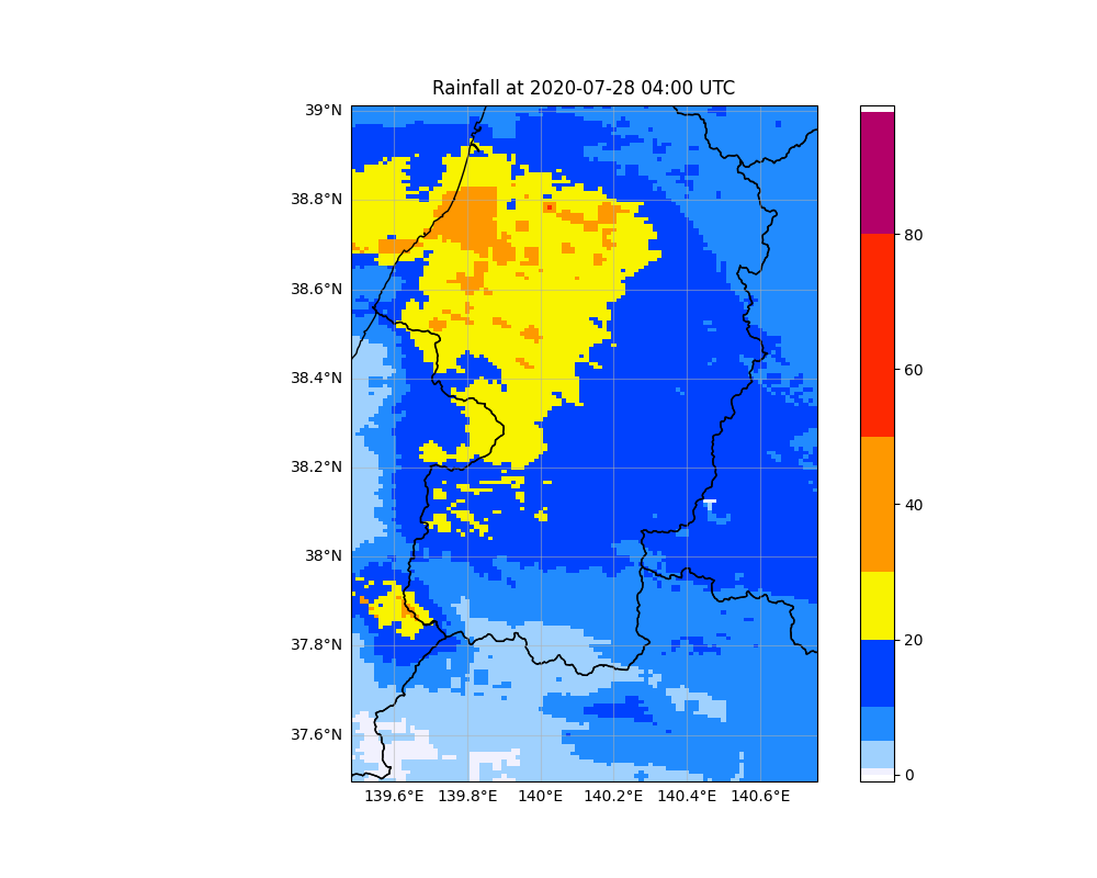
ここでは、Pythonを使って次のような図を作る例を示します。この図は、2020年7月28日04時UTC(日本時間13時)の山形県付近の降雨分布を示したものです。
-
地図データをダウンロードします。
- 地図に市町村の境界を表示する場合は、国土数値情報から 全国の行政区域データ をダウンロードします。ダウンロードした ZIP ファイルに含まれる geojson (たとえば 令和5年のデータなら "N03-23_230101.geojson")を保存します。
- 地図に都道府県の境界を表示する場合は、japonyol.net さんの 47都道府県のポリゴンデータ を使わせていただきます。 geojson を "prefectures.geojson" として保存します。
-
次のコードを "PlotRainfallNc.py" として保存します。
 1
 2
 3
 4
 5
 6
 7
 8
 9
10
11
12
13
14
15
16
17
18
19
20
21
22
23
24
25
26
27
28
29
30
31
32
33
34
35
36
37
38
39
40
41
42
43
44
45
46
47
48
49
50
51
52
53
54
55
56
57
58
59
60
61
62
63
64
65
66
67
68
69
70
71
72
73
74
75
76
77
78
79
80
81
82
83
84
85
86
87
88
89
90
91
import glob import sys from matplotlib.colors import ListedColormap import netCDF4 import numpy as np import matplotlib.pyplot as plt import geopandas as gpd import cartopy.crs as ccrs import datetime as dt # 市町村の境界を表示する場合 # 国土数値情報 行政区域データ # https://nlftp.mlit.go.jp/ksj/gml/datalist/KsjTmplt-N03-v3_1.html # geojson = "N03-23_230101.geojson" # 都道府県の境界を表示する場合 # japonyol.net > 47都道府県のポリゴンデータ geojson # "ダウンロードのうえ使用して下さい。連絡は不要です。" # https://japonyol.net/editor/article/47-prefectures-geojson.html # https://japonyol.net/editor/article/geo/prefectures.geojson geojson = "prefectures.geojson" df = gpd.read_file(geojson) # 気象庁のカラーマップ # https://www.jma.go.jp/jma/kishou/info/colorguide/HPColorGuide_202007.pdf jmacolors=np.zeros((100,4),dtype=float) jmacolors[0:1, :] = [255, 255, 255, 0] jmacolors[1:2, :] = [242, 242, 255, 1] jmacolors[2:6, :] = [160, 210, 255, 1] jmacolors[6:11, :] = [33, 140, 255, 1] jmacolors[11:21, :] = [0, 65, 255, 1] jmacolors[21:31, :] = [250, 245, 0, 1] jmacolors[31:51, :] = [255, 153, 0, 1] jmacolors[51:81, :] = [255, 40, 0, 1] jmacolors[81:99, :] = [180, 0, 104, 1] jmacolors[:, 0:3] /= 256 jmacolors[:, 3] *= 1 jmacmap = ListedColormap(jmacolors) files = glob.glob(sys.argv[1]) cached = False for file in files: nc = netCDF4.Dataset(file) precip = nc.variables['precip'] if (cached == False): lat = nc.variables['lat'] lon = nc.variables['lon'] dummy = np.zeros((lat.shape[0], lon.shape[0]), dtype=float) - 1 time = nc.variables['time'] timeLen = time.shape[0] dlon = lon[1] - lon[0] x = [lon[0] + dlon * (i - 1) for i in range(lon.shape[0] + 1)] dlat = lat[1] - lat[0] y = [lat[0] + dlat * (j - 1) for j in range(lat.shape[0] + 1)] fig = plt.figure(figsize=(10, 8), facecolor="w") ax = fig.add_subplot(1,1,1,projection=ccrs.PlateCarree()) pcm = ax.pcolormesh(x, y, dummy, cmap=jmacmap, vmin=-1, vmax=99) ax.set_xlim(min(x), max(x)) ax.set_ylim(min(y), max(y)) pst = ax.set_title(" ") plt.colorbar(pcm, ax=ax) ax.set_xticks([]) ax.set_yticks([]) gl = ax.gridlines(draw_labels=True,alpha=0.5) gl.top_labels=False gl.right_labels=False df.plot(facecolor='none', ax=ax) bg = fig.canvas.copy_from_bbox(fig.bbox) ax.draw_artist(pcm) fig.canvas.blit(fig.bbox) cached = True for ti in range(timeLen): fig.canvas.restore_region(bg) pcm.set_array(precip[ti,:,:]) t = dt.datetime.utcfromtimestamp(time[ti]) ax.draw_artist(pcm) title = f"Rainfall at {t.strftime('%Y-%m-%d %H:%M')} UTC" pst = ax.set_title(title) fig.canvas.blit(fig.bbox) fig.canvas.flush_events() pngName = f'{file[:-3]}.{ti:04}.png' plt.savefig(pngName) print(pngName) -
Pythonを実行します。第1引数として、可視化対象の netcdf ファイルを開きます。たとえば、"rainfall.nc" を可視化したい場合は次のように呼び出します。
1Python.exe PlotRainfallNc.py rainfall.nc
なお、このスクリプトで可視化の対象とする netCDF の構造の例を示します。
これは、DioVISTA で降雨データとしてインポート可能な netCDFの構造です。
1 2 3 4 5 6 7 8 9 10 11 12 13 14 15 16 17 18 19 20 21 22 23 24 25 26 27 28 29 30 31 32 33 34 35 36 37 38 39 40 41 42 43 44 | |
関連項目
最終更新日:
2024-12-09